Tutorial: Get started with the AutoEMX GUI

The AutoEMX GUI lets you run all of AutoEMX by pointing and clicking: acquire spectra with the microscope, quantify them, identify the phases of your samples with the clustering analysis and explore the results in interactive 3D plots, and fit single spectra. It runs the same engine as the scripts and reads and writes the same sample folders, so you can switch between the GUI and the scripts at any time.

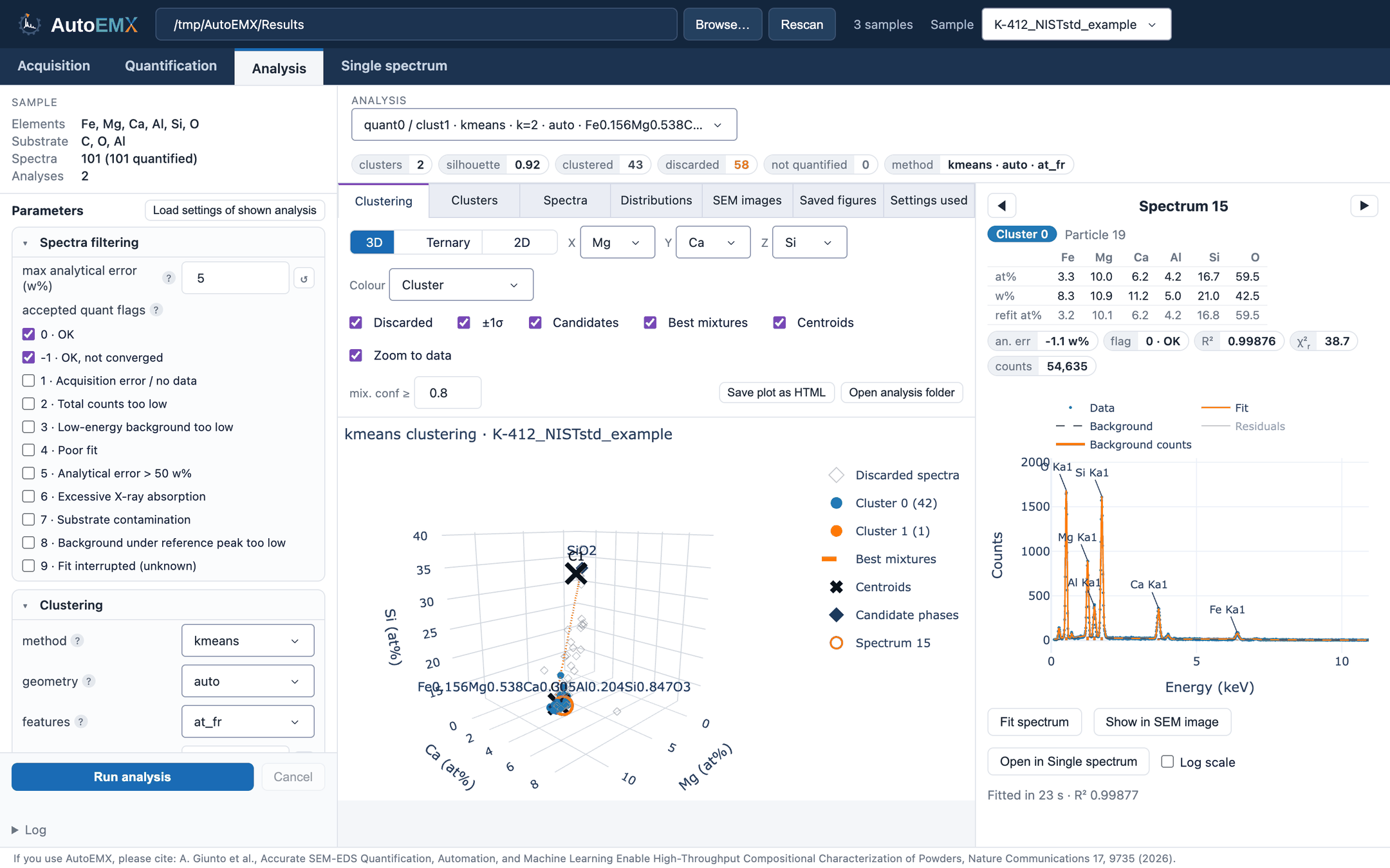
The Analysis tab of the AutoEMX GUI, with the clustering of the K-412 NIST glass standard (example sample K-412_NISTstd_example in examples/Results): interactive 3D plot of the compositions on the left, and a spectrum and its fit on the right.

It runs locally: a small server on your computer (127.0.0.1) shows the interface in your browser. It reads and writes the sample folders on your disk, and nothing is uploaded anywhere.

Note

Try it online. A public demo of the single-spectrum fit and quantification, with no installation, is at https://autoemx-singlespectrum.streamlit.app. It is a demo only: slow, it may need to wake up, it accepts a limited number of files, and it uses the PhenomXL standards at 15 kV.

Step 1 - Create the AutoEMX app (once)

In a terminal, in the Python environment where AutoEMX is installed (see Installation), run:

python -m autoemx.gui --create-launcher

This writes an AutoEMX launcher on your Desktop: AutoEMX.command on macOS (with the AutoEMX icon, shown without its extension), an AutoEMX shortcut with the AutoEMX icon on Windows (it runs a .bat file kept in .autoemx\launchers in your user folder), or AutoEMX.sh on Linux. It replaces a launcher created by an earlier version (AutoEMX GUI). From then on, double-click it to open the GUI, without a terminal. It runs the GUI with the Python environment used to create it, so run the command again if you change environment.

Options: add a results folder to open it directly (python -m autoemx.gui path/to/Results --create-launcher), or a destination folder after --create-launcher to write the launcher elsewhere.

Step 2 - Launch the GUI

Double-click AutoEMX on your Desktop. The interface opens in your browser (http://127.0.0.1:8050). The window that opens with it shows the log, and closing it stops the GUI. Double-clicking again while the GUI runs just reopens it in the browser.

The GUI can also be started from a terminal:

python -m autoemx.gui path/to/Results

with --port 8051 to use another port and --no-browser to not open a browser tab.

Step 3 - Choose the results folder

At the top of the page, choose the results folder of your project with Browse… (or type its path). It is the folder containing one sub-folder per sample, as written by the acquisition (results_dir in the scripts); sub-folders are searched as well. Rescan looks for new samples. The Sample menu next to it selects the current sample, shared by all tabs.

What the GUI can do

The GUI has four tabs:

• Acquisition: acquire the spectra of a list of samples with the microscope, with every option of the acquisition script, and optionally quantify them during acquisition. Use it on the microscope computer.

• Quantification: quantify the spectra of one or more samples (or only of the samples just added to a project), and optionally analyse them right after. It also imports folders of spectra acquired without AutoEMX (.msa, .emsa, .msg), to quantify and analyse them like the others.

• Analysis: run the clustering analysis of a sample with every parameter, and explore the results: interactive 3D, ternary and 2D plots of the compositions, clusters and candidate phases, tables of clusters and spectra, element distributions, the SEM images with the position of every spectrum, and the figures saved by the analysis. Click any point to see its spectrum, fit it, or find it on the SEM image.

• Single spectrum: fit and quantify one spectrum, of a sample or from an exported file, with every fitting option, and inspect the fit peak by peak.

To learn how to use them, follow:

• Tutorial: EDS compositional analysis for phase identification in the GUI: acquisition, quantification and analysis of samples (Acquisition, Quantification and Analysis tabs).

• Tutorial: Fit and quantify individual spectra in the GUI: fit and quantify individual spectra, one at a time or in batch, from AutoEMX or from other instruments (Single spectrum and Quantification tabs).

Helpful features shared by all tabs:

• ? next to a parameter shows its description.

• ↺ next to an optional field empties it, i.e. goes back to its default or saved value.

• Quantifiable elements (Acquisition and Quantification tabs) shows the periodic table of the elements with P/B standards for a microscope and beam energy. Elements without standards in your samples are also flagged below the samples table.

• Long tasks (acquisition, quantification, analysis, fits) run in the background, with their log and a Cancel button; you can keep using the other tabs meanwhile. Only one task writing to the samples (acquisition, quantification, analysis, import) runs at a time.

• The Quantification table reads the ledger of every sample; on cloud drives, ledgers not stored locally can take a few seconds each to download the first time. Summaries are cached in ~/.autoemx/gui_sample_summaries.json and only re-read when a ledger changes.

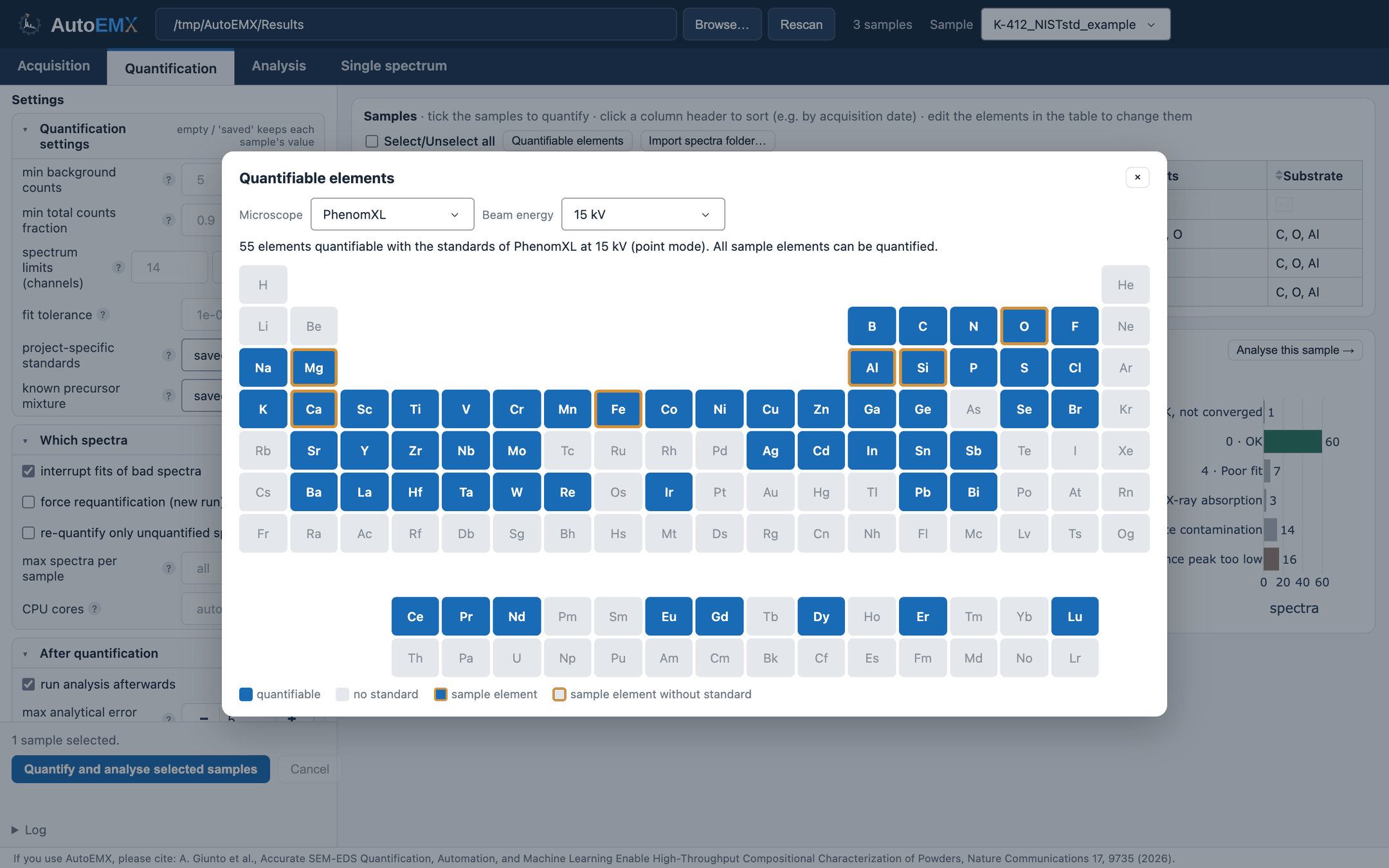
Quantifiable elements: elements with P/B standards for the PhenomXL at 15 kV. The elements of the ticked sample (here K-412) are outlined in orange.