Tutorial: Fit and quantify individual spectra in the GUI

This tutorial shows how to fit, and optionally quantify, EDS spectra in the AutoEMX GUI: one spectrum at a time, to inspect the fit in detail, or many spectra in batch; acquired with AutoEMX or exported by commercial EDS software (.msa, .emsa, .msg files). It is the GUI equivalent of Tutorial: Fit and quantify individual spectra acquired with AutoEMX, Tutorial: Fit and quantify individual spectra exported by commercial EDS software and Tutorial: Quantify externally exported spectra in batch.

If you have not opened the GUI yet, start with Tutorial: Get started with the AutoEMX GUI.

Spectra	Where
One spectrum of an AutoEMX sample	Single spectrum tab, or Fit spectrum in the Analysis tab
One exported spectrum file	Single spectrum tab, External file
Many spectra of AutoEMX samples	Quantification tab
A folder of exported spectra	Quantification tab, Import spectra folder…

Fit one spectrum

The Single spectrum tab fits and quantifies one spectrum with every option of the single-spectrum scripts, and shows the fit peak by peak. Results are only shown: they are not saved to the sample’s ledger.

Step 1 - Choose the spectrum

• Spectrum of the current sample: a spectrum acquired with AutoEMX. Choose the sample at the top of the page and the spectrum in the menu (or with ◀ / ▶). From the Analysis tab, click a point of the plot and then Open in Single spectrum to open it here.

• External file: a spectrum exported by commercial EDS software, chosen with Browse… or dropped on the page. Its beam energy, emergence angle, live time and energy calibration are read from its header. It is quantified with the P/B standards of the default microscope (PhenomXL), which exist at 15 kV only: compositions of spectra acquired at other voltages are not valid.

The raw spectrum is shown as soon as it is chosen.

Step 2 - Set the fit and quantification options

For spectra of a sample, the options are filled in with the settings of the sample’s active quantification; Use sample settings restores them.

Elements:

• known sample elements: elements known to be in the sample, quantified. Elements giving peaks but not listed (in the sample or substrate elements) distort the fit, unless identify missing elements is ticked.

• known substrate elements: elements fitted but not quantified, e.g. C, O, Al for carbon tape on an Al stub. Their peaks are never attributed to the sample, not even by identify missing elements: list only elements you do not want quantified. To quantify an element also present in the substrate (e.g. O in an oxide), list it among the known sample elements.

• standard of known composition and standard formula: the spectrum is from a standard of known composition: report its measured P/B ratios. For spectra of a sample, an empty formula uses the composition saved in the ledger.

Fit and quantification:

• quantify: untick to only fit the spectrum, without quantifying it.

• identify missing elements: before the fit, look for peaks of elements missing from the known elements (which may then be empty). Elements surely present are added: quantified if a standard is available, otherwise only fitted. Doubtful ones are only reported. The result is shown in the element check field above the composition. On by default (slower); for spectra of a sample, it follows the setting of the sample’s active quantification.

• particle geometry: tick for particles and powders, untick for bulk or flat samples.

• fit tolerance: tolerance for the convergence of the fit.

• spectrum limits: first and last channel of the fitted range. Empty uses the saved value (or the default, for external files).

• max undetectable mass fraction: maximum mass fraction of elements not detectable by EDS (e.g. Li); the total of the fitted elements is constrained between 1 minus this value and 1.

• single iteration: run a single fit and quantification iteration.

• interrupt fit of bad spectra: stop early on spectra expected to give large errors.

• free-area lines: X-ray lines fitted with a free area, e.g. Fe_La, for lines poorly described by the model.

Step 3 - Fit and inspect the results

Click Fit and quantify (or Fit spectrum when quantify is off). It takes about 10–30 s. Then:

• The plot shows the data, the fit, the background, the background counts under the reference peaks and the residuals, over the fitted range. Zoom to line zooms on any fitted line; tick Log scale to see weak peaks.

• Below are the fit quality (R², reduced χ²), the analytical error and the quant flag (see Quantification flags (quant_flag)); the composition (atomic and mass fractions) and, for spectra of a sample, the composition saved in the ledger for comparison.

• The fitted peaks table gives the energy, FWHM, area, height and P/B ratio of each line. Download CSV saves the composition or the peaks.

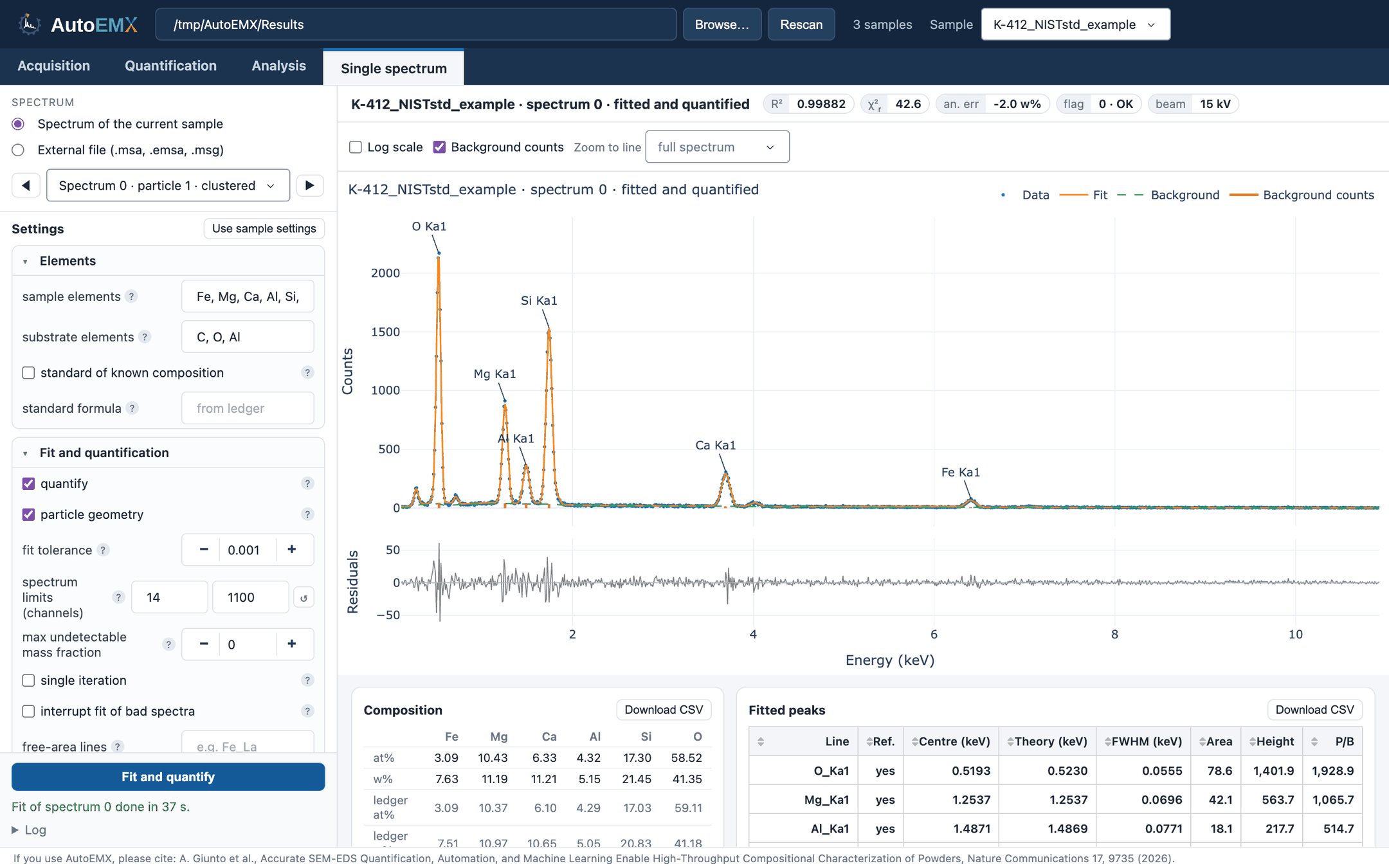
A spectrum of the K-412 example fitted and quantified in the Single spectrum tab: data, fit, background and residuals, with the composition and the fitted peaks below.

For a quick check of a spectrum while exploring an analysis, Fit spectrum under the spectrum panel of the Analysis tab re-fits it with the settings of the active quantification, without leaving the tab.

Fit and quantify many spectra

Many spectra are quantified in the Quantification tab. Unlike the Single spectrum tab, the results are saved to the ledger of each sample, so that the samples can then be analysed in the Analysis tab.

Spectra acquired with AutoEMX

Tick the samples in the table and click Quantify selected samples (or Quantify and analyse selected samples). See Step 9 of Tutorial: EDS compositional analysis for phase identification in the GUI for the options. Use max spectra per sample to quantify only the first spectra of each sample, e.g. for a quick test of the settings.

Spectra exported by commercial EDS software

Put the spectra of each sample in a folder, then:

1. Click Import spectra folder… above the samples table, and choose the folder (or type its path). The number of spectra, and the beam energy and energy calibration written in their headers, are shown. The energy calibration is always taken from the headers (#OFFSET and #XPERCHAN); folders without it, or with spectra of different calibrations, cannot be imported.

2. Set:

   • Sample ID: name of the new sample folder (by default, the name of the spectra folder).

   • Known sample elements and known substrate elements (empty if there is no substrate).

   • Sample type: powder, powder_continuous, bulk or bulk_rough.

   • Microscope: its P/B standards are used for the quantification.

   • Beam energy: filled in from the headers.

3. Import copies the spectra into a new sample folder of the results folder and writes its ledger. The original files are not modified.

4. The new sample appears in the samples table: tick it and quantify it as above. With Run analysis afterwards, the clustering analysis runs right after; set the candidate phases and re-run it in the Analysis tab (Step 10 of Tutorial: EDS compositional analysis for phase identification in the GUI).

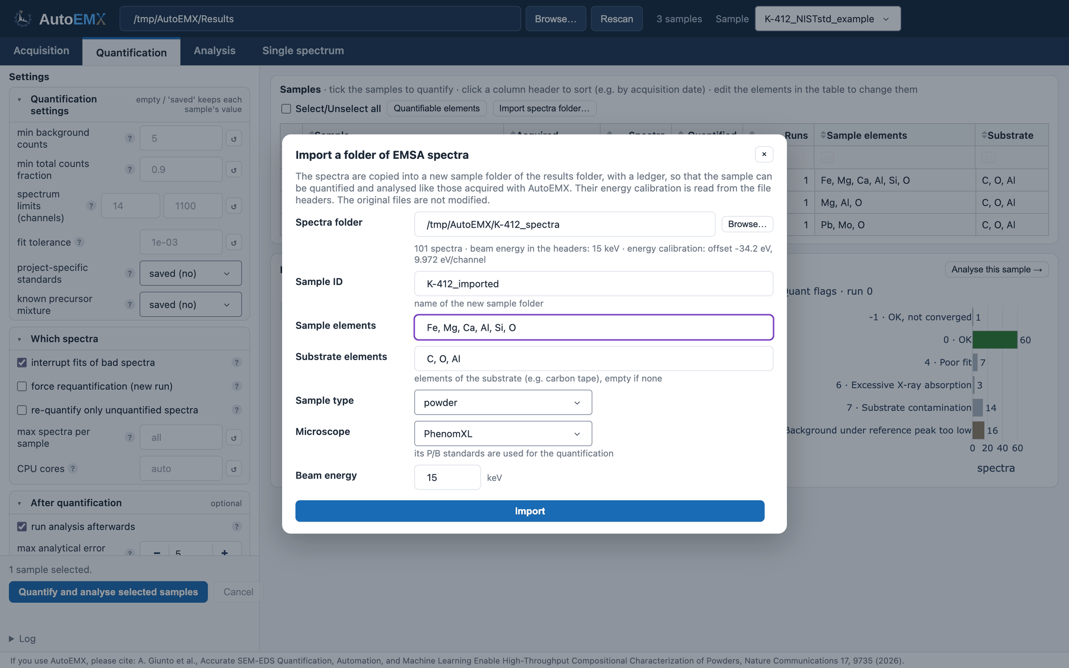
Import spectra folder…: the number of spectra, beam energy and energy calibration are read from the headers of the spectra, here those of the K-412 example.