Tutorial: EDS compositional analysis for phase identification in the GUI

This tutorial shows how to run the automated workflow for EDS compositional analysis in the AutoEMX GUI. It is the GUI equivalent of Tutorial: EDS compositional analysis for phase identification, which uses the Run_Acquisition.py, Run_Quantification.py and Run_Analysis.py scripts.

The workflow is described in Giunto et al., Nature Communications 17, 9735 (2026) (https://doi.org/10.1038/s41467-026-76633-x), and includes:

• Acquisition of EDS spectra from powder or bulk samples (Acquisition tab)

• Fitting and quantification to extract compositions (Quantification tab, or during acquisition)

• Rule-based filtering of compositions, and clustering analysis to detect the number of phases and extract their compositions (Analysis tab, or right after quantification)

Several samples can be acquired and quantified one after the other with a single click.

If you have not opened the GUI yet, start with Tutorial: Get started with the AutoEMX GUI. To analyse spectra acquired without AutoEMX, import them first as described in Tutorial: Fit and quantify individual spectra in the GUI (Fit and quantify many spectra), then continue from Step 7.

Step 1 - Open the Acquisition tab

Open the GUI on the microscope computer and choose the results folder of your project at the top. The Acquisition tab shows whether the microscope API (e.g. PyPhenom for the Phenom XL) is available; the GUI opens on this tab when it is.

In the Microscope section, select the microscope (PhenomXL by default). It sets the driver, the calibrations and the P/B standards used for the quantification. The chips above the form show whether the microscope is connected and whether P/B standards exist at the chosen beam energy. Quantifiable elements shows the periodic table of the elements with standards.

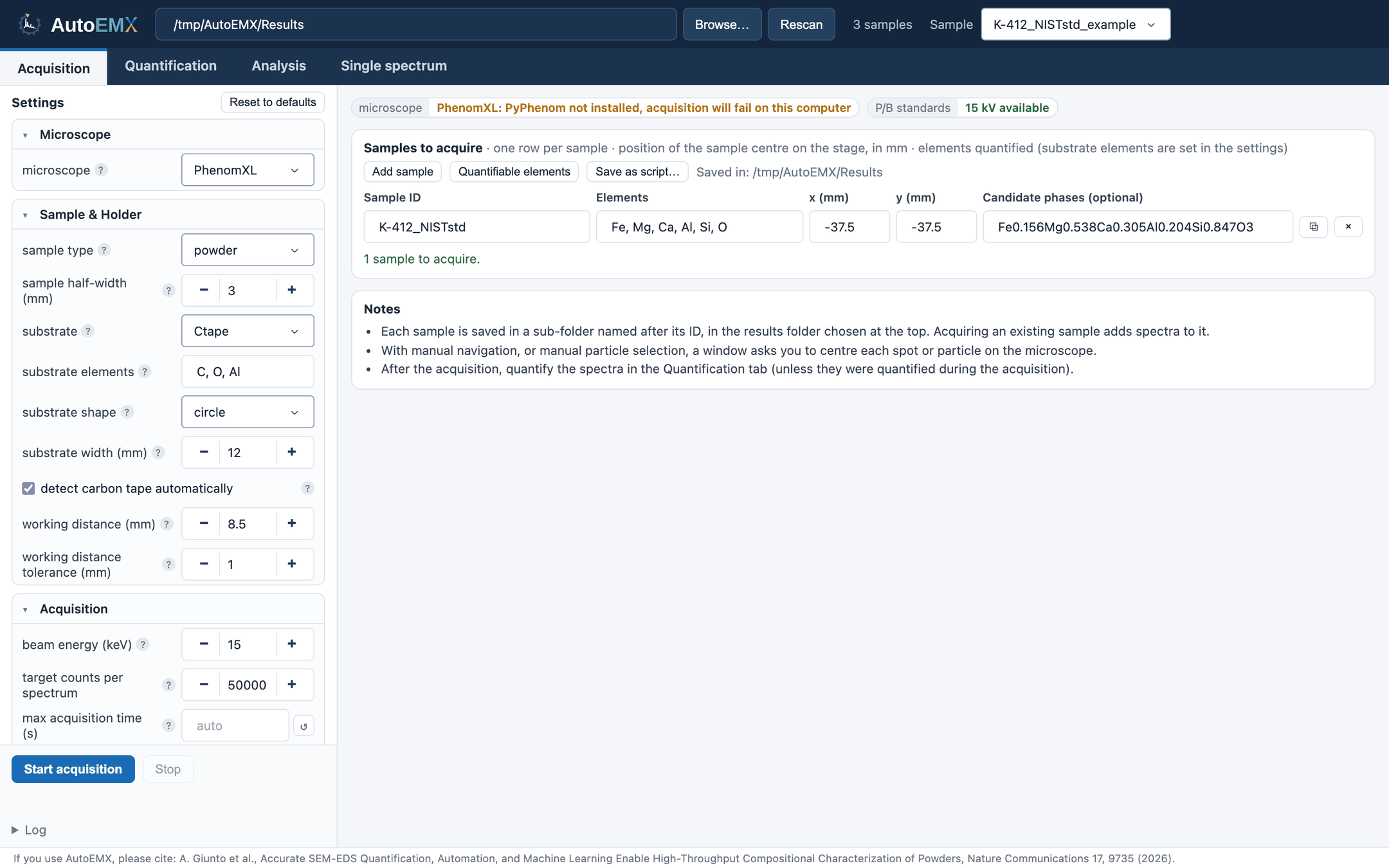
The Acquisition tab, with one sample to acquire (K-412) and its settings. On this computer the microscope API is not installed, as the status chip at the top shows.

Step 2 - Define the samples to analyse

In Samples to acquire, add one row per sample (Add sample; ⧉ copies a row, × deletes one):

• ID: sample identifier. All data are saved in the results folder, under a folder named after the ID. Acquiring a sample that already exists adds spectra to it (Step 8).

• Elements: elements quantified from the EDS spectra. Do not include elements present only in the substrate (e.g. C from carbon tape); these are set in Sample & Holder. Avoid light elements dominant in the substrate even if present in the sample (e.g. C from carbonates on carbon tape), as this may disrupt quantification and lead to large analytical errors. In general, avoid element overlap between substrate and sample. Elements without a P/B standard are flagged below the table.

• x, y: sample centre position in absolute stage coordinates (mm), typically obtained from Saved Positions at the microscope.

• Candidate phases (optional): compositions that may be present, e.g. MgO, Al2O3. They can be changed later when re-running the analysis.

In Sample & Holder, set the parameters common to all samples:

• sample type: powder, bulk, powder_continuous or bulk_rough

• sample half-width: half-width of the sample region to analyse (mm)

• substrate (Ctape or None), substrate elements (e.g. C, O, Al for carbon tape on an Al stub), substrate shape (circle or square) and substrate width (SEM stub diameter, mm)

• detect carbon tape automatically: currently supported only for carbon tape that appears dark on a brighter stub (e.g. Al). Allows to be tolerant to off-centred sticking of the tape.

• working distance: approximate working distance (mm). Autofocus is limited to working distance tolerance around this value, to avoid large focusing errors.

The settings and the sample list are kept in the browser between sessions; Reset to defaults restores the defaults of the script.

Step 3 - Define the measurement settings

In Acquisition:

• beam energy (keV): a P/B standards file must exist for this voltage (see the status chip).

• target counts per spectrum.

• max acquisition time (s): maximum acquisition time per spectrum, after which the acquisition is interrupted and the spectrum discarded.

• manual navigation: manually navigate to the region of interest. Typically off, unless you want to analyse a specific region of the sample.

• automatic brightness/contrast: typically on. When off, set contrast and brightness.

• number of spectra, or min spectra and max spectra when quantifying during acquisition (Step 4).

Warning

max acquisition time should be set as a function of the detector counts/sec, so that the acquisition is interrupted only when wrong regions are selected (e.g. carbon tape or a void in the sample instead of a particle). Spectra interrupted due to this parameter are flagged (quant_flag = 2) and discarded. Make sure it is high enough for your EDS system.

In Images: image format, and whether particle images are annotated with the positions of the spectra (by default they are saved raw: the Analysis tab shows the positions anyway).

Step 4 - Quantify spectra during acquisition

Tick quantify during acquisition to quantify spectra while they are acquired. Quantification is parallelised but may be slow on less powerful microscope computers; in this case, leave it off and quantify the spectra afterwards in the Quantification tab (Step 9), possibly on another computer.

When on, AutoEMX periodically checks for convergence and may stop the acquisition early, between min spectra and max spectra:

• If no candidate phases are assigned: all clusters must have RMS point-to-centroid distance < 2.5%.

• If candidate phases are assigned: confidence score > 0.8 and RMS point-to-centroid distance < 3%.

Step 5 - Define other parameters

The Quantification section of the Acquisition tab is used when quantifying during acquisition. These settings can also be changed later in the Quantification tab, but require re-quantification:

• interrupt fits of bad spectra: interrupt the quantification of spectra expected to lead to large errors. Typically on, to speed up quantification.

• min background counts: minimum counts required under a reference peak. Spectra failing this criterion are flagged (quant_flag = 8). If too many spectra are flagged, decrease it or increase the target counts in your following measurements.

• project-specific standards: use the P/B standards file saved in the results folder.

These only require re-analysis (Analysis tab):

• max analytical error (w%): compositions with a larger analytical error are discarded from the clustering.

• accepted quant flags: flags considered valid in the clustering (see Quantification flags (quant_flag)).

• max clusters: maximum number of clusters; 6 is generally sufficient for materials science samples.

• show discarded compositions: show compositions discarded from the clustering in the plots. Even if discarded because of their analytical error, they can hint at the phases present in the sample.

Step 6 - Sample-type-specific settings

Depending on the sample type, set the Powder acquisition params (detection of particles and choice of the EDS spots on them) or the Bulk grid acquisition params (grid of EDS spots for bulk, bulk_rough and powder_continuous). The section that does not apply is greyed out. See PowderMeasurementConfig and BulkMeasurementConfig for details; the ? next to each field describes it.

Step 7 - Launch spectra acquisition

Start acquisition asks for confirmation, then acquires the samples one after the other, with a progress bar per sample and the log. With manual navigation or manual particle selection, a window asks you to centre each spot or particle. Stop interrupts the acquisition, keeping the spectra already acquired; the microscope is left in its current state. When the acquisition ends, the results folder is rescanned and the new samples appear in the other tabs.

Save as script… downloads a Python script running the same acquisition, e.g. to run it on the microscope computer without the GUI.

The sample folders contain the same output as with the script: SEM images, spectra and ledger.json (see Output in Tutorial: EDS compositional analysis for phase identification).

Step 8 - Optional: (re)acquire spectra

You can restart an interrupted acquisition, or acquire more spectra after inspecting the first results: start the acquisition again with the same sample ID. AutoEMX resumes from the next available spectrum and particle IDs. See Restarting acquisition in Tutorial: EDS compositional analysis for phase identification for how existing spectra are handled.

Step 9 - Optional: (re)quantify spectra

This step is done automatically if you quantified during acquisition. Otherwise, or to quantify again with other settings, use the Quantification tab, on the microscope computer or on a more performant one (e.g. with more CPU cores) with access to the results folder.

1. Tick the samples to quantify in the table. All samples start unticked, so you can quantify only the samples just added to a project. Sort the table by clicking a column header, e.g. Acquired to show the latest samples first, and filter it by typing in the row below the headers. Select/Unselect all ticks (or unticks) all the samples listed.

2. Elements. The known sample and substrate elements of each sample can be edited in the table. Unchanged elements keep the values saved in the sample’s ledger.

3. Settings. Options left empty (or set to saved) keep each sample’s saved value. When the ticked samples share the same saved value, it is shown in grey in the empty field (and as e.g. saved (no) in the menus); saved means that their values differ. Identify missing elements: before fitting each spectrum, look for peaks of elements missing from the known elements. Elements surely present are added to that spectrum (quantified if a standard is available, otherwise only fitted); doubtful ones are only reported. The elements found are listed per spectrum (Added elements and Possible elements columns of Compositions.csv), per sample (Element_identification_report.txt) and per batch (at the end of the log). On by default (slower); quantification runs saved before this option existed keep it off. Which spectra: interrupt fits of bad spectra, force requantification (new quantification run), re-quantify only unquantified spectra (e.g. after lowering the minimum background counts), and max spectra per sample to quantify only the first N spectra, e.g. for a quick test. CPU cores: number of cores used in parallel (half of the available cores by default). Run analysis afterwards (on by default) runs the clustering analysis right after the quantification.

4. Quantify and analyse selected samples (or Quantify selected samples). The samples are quantified one after the other, in the order of the table, with a progress bar per sample and the log. Cancelling keeps the spectra already quantified.

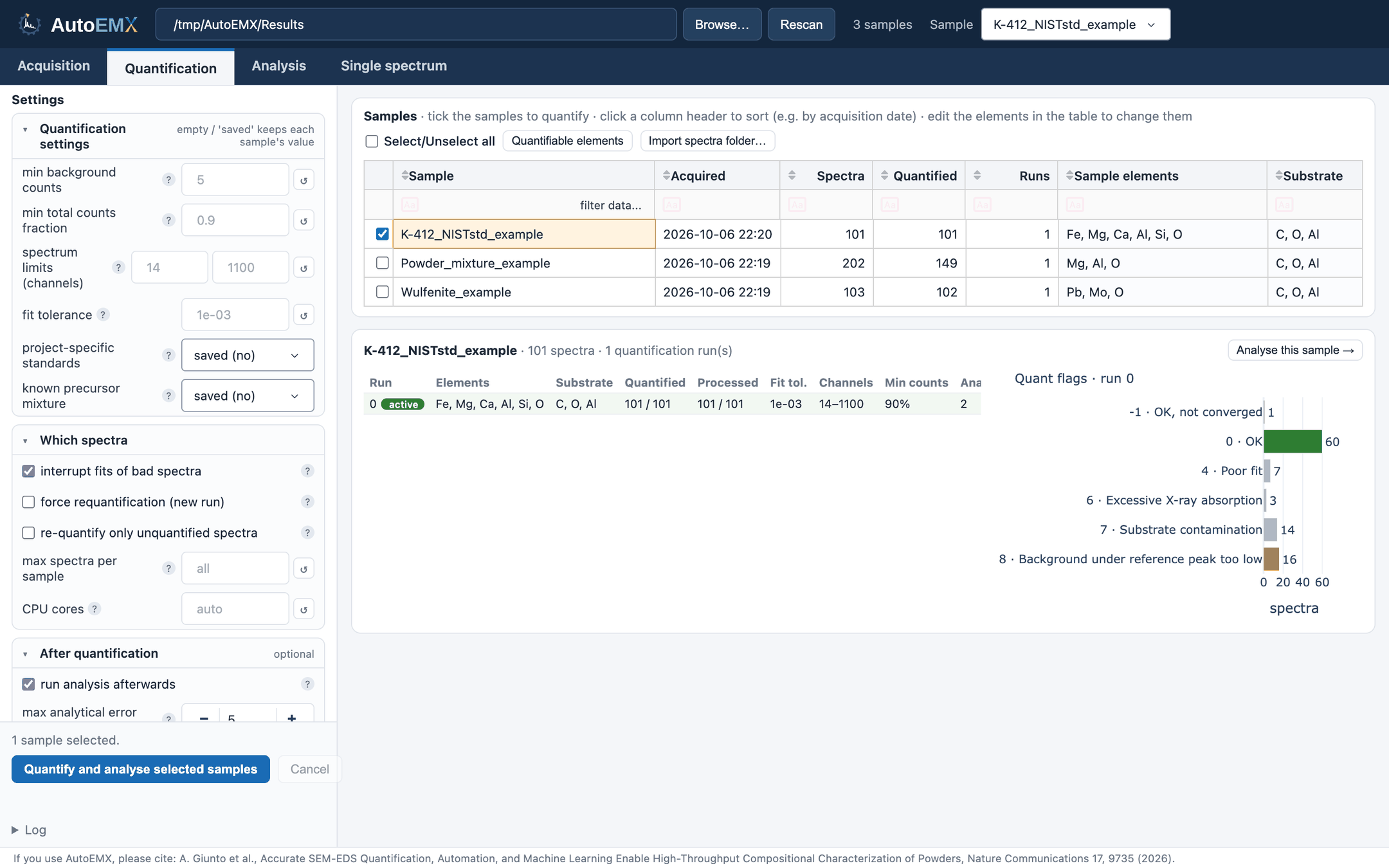
The Quantification tab, with the K-412 sample ticked. Below the table, its quantification runs and the quant flags of the active run.

Click a sample in the table to show its quantification runs (settings, number of quantified spectra, quant flags; see Quantification flags (quant_flag)) and the flags of its active run. Analyse this sample → opens it in the Analysis tab.

Step 10 - Optional: (re)analyse spectra

This step is done automatically if you quantified during acquisition, or with Run analysis afterwards. To run the analysis again with other parameters, open the Analysis tab.

1. Select a sample at the top. The sidebar shows its elements, substrate, number of spectra and of quantified spectra. The latest (active) analysis is shown.

2. Set the parameters. The form contains every clustering parameter, filled in with the values saved in the sample’s ledger. Parameters not used with the current settings are greyed out. Load settings of shown analysis fills the form with the settings of the analysis selected above the plot. Set as active makes the selected analysis the active one: its settings are then reused by later analyses and it is shown by default.

   • Spectra filtering: maximum analytical error, minimum background counts (quant flag 8, applied without re-quantifying) and accepted quant flags.

   • Clustering: method (k-means or DBSCAN), geometry (euclidean, Aitchison or auto; see Clustering modes), features (atomic or mass fractions), number of clusters (empty = found automatically, with the chosen method), candidate phases, and mixture decomposition.

   • DBSCAN, Aitchison geometry, Cluster merging, Mixture decomposition: all their parameters (see Mixture decomposition and the mixture options in Tutorial: EDS compositional analysis for phase identification).

   • Plot output: options of the PNG figures saved in the analysis folder (elements on the axes or excluded from the plot, discarded compositions, custom plots).

3. Run analysis. The analysis runs in the background (a few seconds) and can be cancelled. Results are saved to the ledger and to an analysis_quant<i>_clust<j> folder, exactly as with the script.

4. Explore the results.

   • Clustering: 3D, ternary (3 elements, normalised) or 2D plot of the compositions, with clusters, ±1σ ellipsoids, centroids, candidate phases and the best mixture of each cluster (shown when its confidence is at least mix. conf). Choose the elements on each axis, colour the spectra by cluster, analytical error, particle, quant flag or R², and toggle each layer. Rotate and zoom with the mouse; click legend entries to hide them. Save plot as HTML saves the interactive plot in the analysis folder.

   • Clusters: composition ± standard deviation of each cluster, candidate phases and mixtures with their confidence and molar fractions (the content of Clusters.csv).

   • Spectra: table of all spectra, sortable and filterable.

   • Distributions: fraction of each element by cluster.

   • SEM images (named after the microscope type): the image of the particle (or frame) where the selected spectrum was collected, with all spectrum spots marked and coloured by cluster (click a spot to select its spectrum). ◀ / ▶ step through the images, which are also shown in a strip below, sorted by particle number.

   • Saved figures and Settings used: the PNG figures and Analysis_config_summary.txt of the analysis.

5. Inspect single spectra. Click a point in the plot, a row of the table or a point of the distributions to show the spectrum and its composition on the right; ◀ / ▶ browse through the spectra. Show in SEM image opens the image where it was collected, with its spot highlighted. Fit spectrum re-fits it (about 10 s) to show the fitted model, the background and the background counts under the reference peaks. Open in Single spectrum opens it in the Single spectrum tab, to fit it with other settings (see Tutorial: Fit and quantify individual spectra in the GUI).

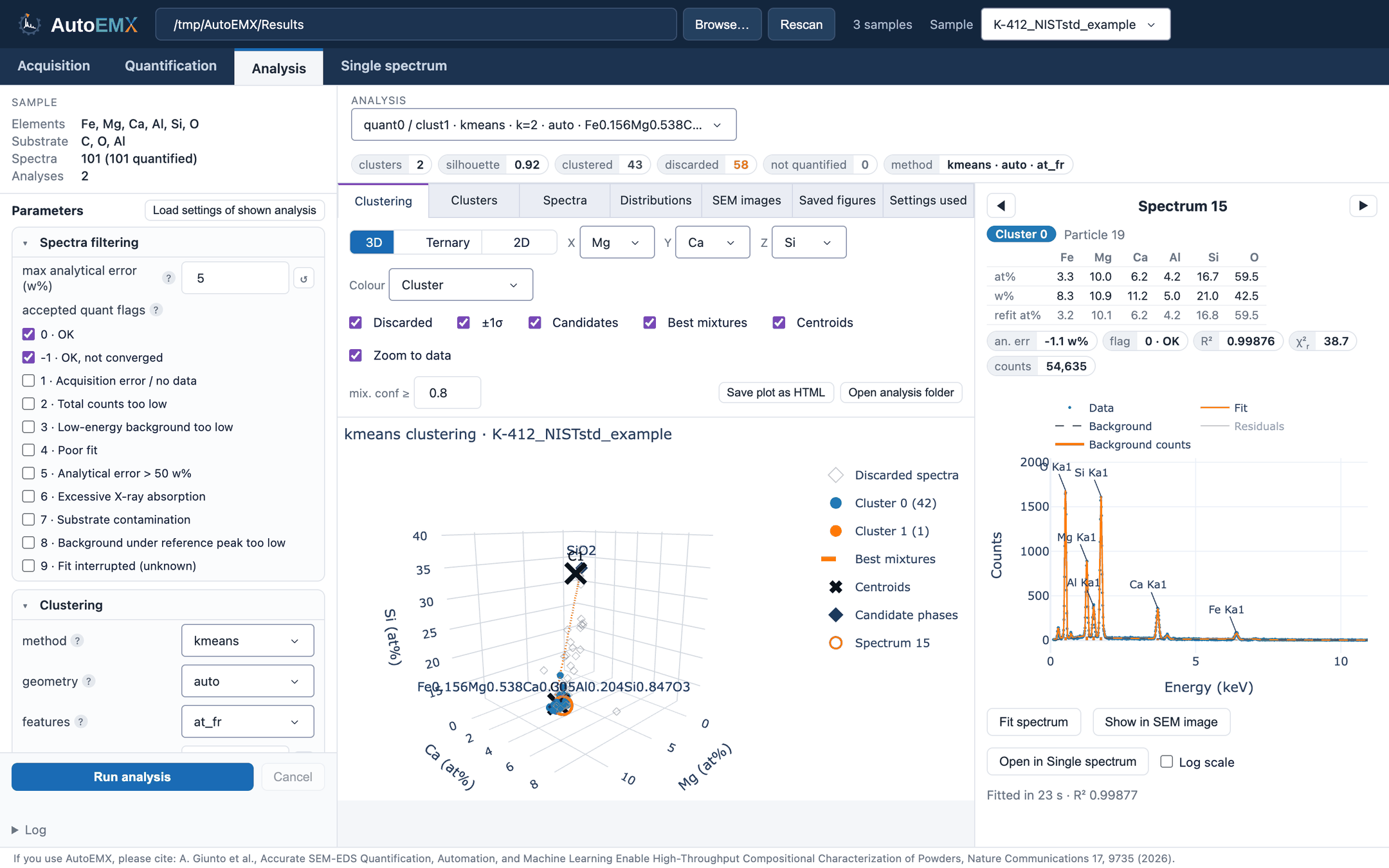
Clustering of the K-412 NIST glass standard (example sample K-412_NISTstd_example in examples/Results), with Zoom to data on. Spectrum 15 is selected in the plot and fitted with Fit spectrum (right). Grey diamonds are spectra discarded by the filters.

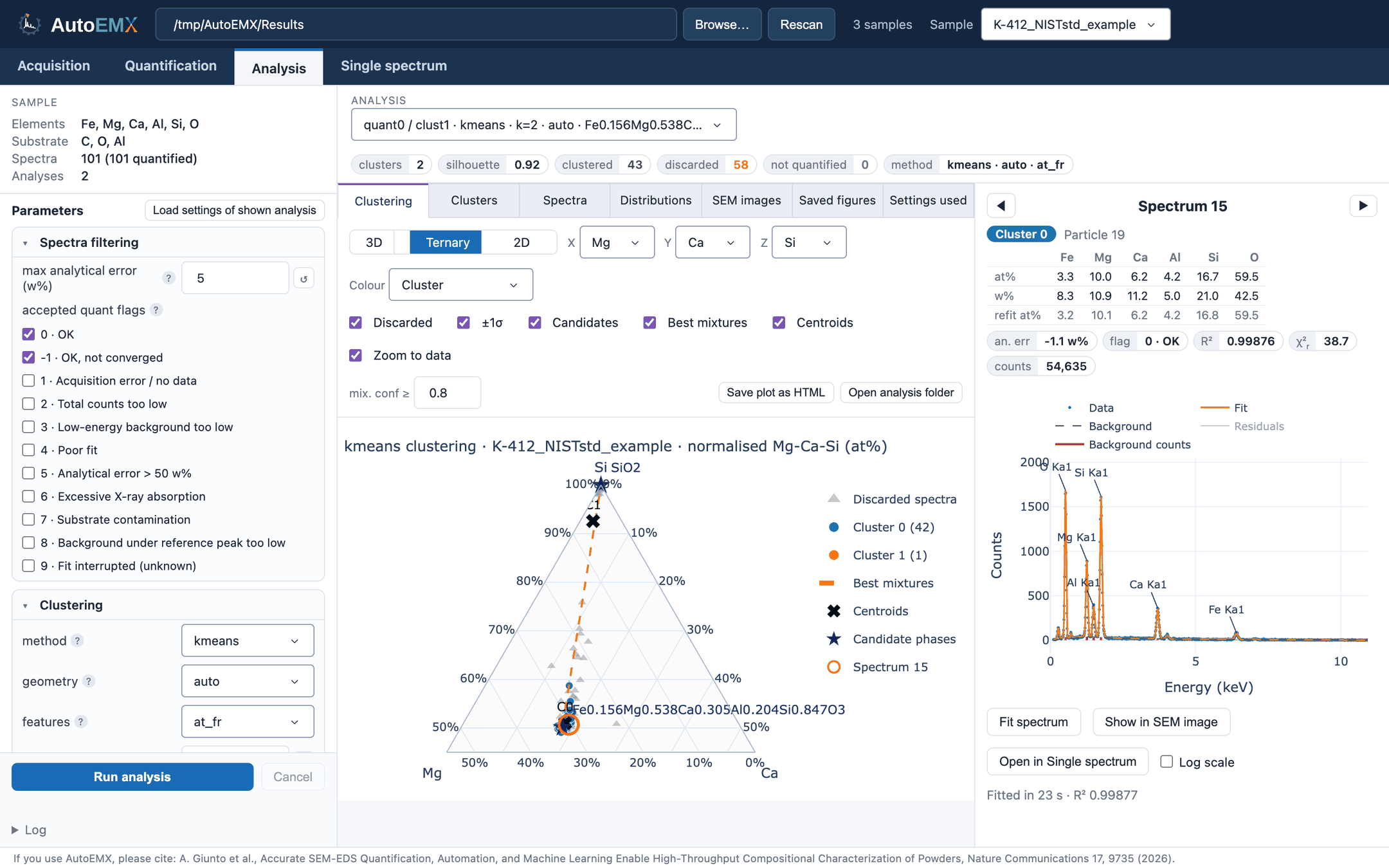
The same analysis as a ternary plot of Mg, Ca and Si (normalised atomic fractions), with the candidate phases and the best mixture of each cluster.

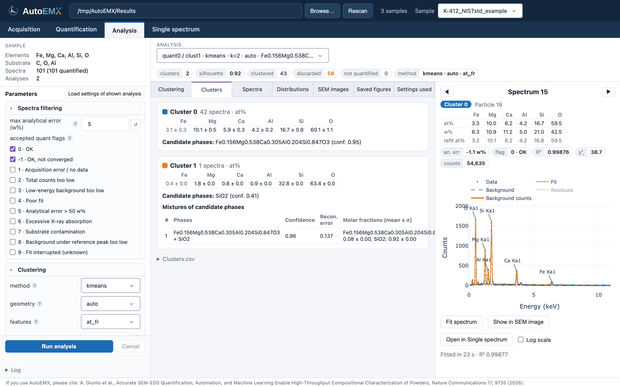
The Clusters view: composition of each cluster, matching candidate phases and mixtures of candidate phases, with their confidence.

Previous analyses of a sample can be selected in the Analysis menu above the plot.

Quantify the extent of intermixing in precursor powders

The GUI also runs the workflow of Tutorial: Quantify the extent of intermixing in precursor powders, which follows the steps above with these differences:

• In Step 2, give only the two intermixed compositions as candidate phases.

• In Step 5, tick project-specific standards to use the standards of the precursors saved in the results folder (see Step 1 of Tutorial: Quantify the extent of intermixing in precursor powders); without them, the default standards are used.

• In Step 6, tick is known powder mixture measurement in the powder acquisition parameters. It can be changed later with known precursor mixture in the Quantification tab.

The violin plots of the molar fractions of the precursors appear under Saved figures in the Analysis tab.