Particle size statistics
How AutoEMX turns the particles measured in SEM frames into statistics of the sample. To run a measurement, see the tutorials in the GUI or with scripts.
Size bands
Particle size is the area-equivalent diameter, \(d = 2\sqrt{A/\pi}\). A frame
only measures particles covering at least min_par_pixels pixels (default 80,
~10 pixels across) and at most a tenth of its width. Wider size ranges are split
into size bands, planned from the smallest particles up, the hardest to find:
each band uses the largest frame (up to 500 µm) in which its smallest particles
still have enough pixels. n_par_target particles are collected in each band.
Segmentation models
Particles are found in each frame by a segmentation model (par_segmentation_model):
threshold_bright(default): pixels brighter thanpar_brightness_thresh. Fast, but only suited to samples without particle aggregation: touching particles are always counted as one.SAM2[Ravi2024] andmicroSAM[Archit2025]: segment each particle on its own, also when touching. Optional, install withpip install "autoemx[segmentation]"(SAM2) orpython -m autoemx.utils.install_segmentation micro-sam(microSAM; ignore pip’s warnings about PyQt6, segment-anything-py and trackastra). Agglomerates, surface features and particles partly hidden by others are left out. Model options go inpar_segmentation_params, e.g.{"pred_iou_thresh": 0.7}.Your own model (see the particle size tutorial).
As general advice, SAM2 follows the outline of irregular particles more closely, while
micro-sam separates rounded particles in agglomerates better. Results vary with the sample,
so try both: segment the frames again with the other model and compare (in the GUI:
Segment again; with scripts: Reanalyse_Particle_Stats.py and
Process_Particle_Stats_Files.py). Each model gives its own result; choose the one that best
matches the particles in the frames.
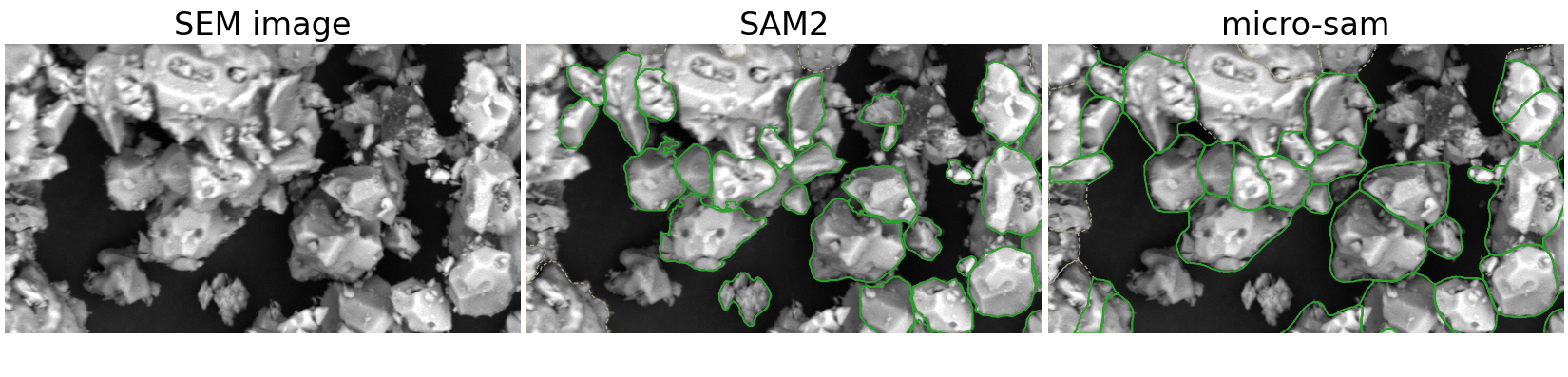
Irregular particles (detail of a frame): SAM2 follows their jagged outlines, while micro-sam rounds them and merges some neighbouring particles. Counted particles in green; particles not counted (cut by the frame edge, or outside the size range) dashed in amber.
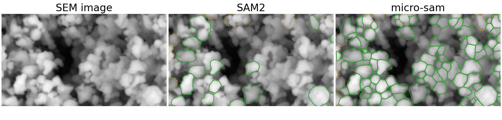
Agglomerates of rounded particles (detail of a frame): micro-sam separates nearly every particle (366 counted in the frame), SAM2 only a few (30).
Corrections
Each particle gets a weight, so that the statistics describe the sample and not the way it was imaged:
Frame edge. Particles touching the frame edge are left out, which would under-count large particles. Each measured particle (bounding box \(w \times h\) in a \(W \times H\) frame) is counted \(c = WH / ((W-w-7)(H-h-7))\) times, the Miles-Lantuéjoul correction [Miles1974] [Lantuejoul1978].
Scanned area. Each particle counts \(c\) divided by the area of the frames able to measure its size, so that each size counts in proportion to its particles per unit area, not to the number collected.
EDS. The frames searched by EDS (automatic particle selection) on the same sample count as extra area, with all the particles in them (
include_eds_auto_particles). A sample measured only by EDS also gets statistics.Overlapping frames counting the same particle sizes are counted once, keeping the largest frame.
The unweighted statistics are kept in ledger.json for comparison.
Reported statistics
All sizes are equivalent diameters, in µm. The GUI (Analysis > Particle sizes) and
<sample>_Par_size_stats.csv report:
Particles: number of particles measured.
Mean, Std. dev., Min, Max: of the diameters.
D10, D25, D50, D75, D90 (number-weighted): the diameters below which 10, 25, 50 (the median), 75 and 90 % of the particles are.
D[4,3], Dv10, Dv50, Dv90 (volume-weighted, for comparison with laser diffraction): each particle counted as a sphere, in proportion to \(d^3\).
D43is the volume-weighted mean diameter, \(D[4,3]\) [ISO9276]; Dv10, Dv50 and Dv90 are the diameters below which 10, 50 and 90 % of the particle volume is. They are dominated by the largest particles and need many more of them to be precise.Span (D90-D10)/D50 (Compare samples): the width of the distribution.
Columns:
Weighted: with the corrections above, describing the sample. Use these.
95 % CI: 95 % confidence interval of the weighted value, by bootstrap [Efron1993] (the frames of each band are resampled, with their particles and area). Given once each band has 5 frames.
Unweighted: plain statistics of the particles measured, for comparison.
The plot shows the weighted number fraction of particles per diameter bin, the cumulative number and volume distributions, and D10, D50 and D90. The Size bands table gives, per band, its diameters, frame width, number of frames, area scanned, particles, and particles per mm²; Frames searched by EDS the same for the frames searched during an EDS acquisition.
Weighted percentiles use type 5 of Hyndman and Fan [Hyndman1996].
Stopping on precision
Set size_stats_ci_tolerance (e.g. 0.05) to collect particles until the
confidence interval of size_stats_ci_quantities (default ["D50"]) is within
± that fraction, up to size_stats_max_n_frames frames (default 500).
n_par_target is then the minimum per band.
Output
ledger.json, <sample>_Par_sizes.csv (each particle with its frame, its
number in the frame and its Weight), <sample>_Par_size_stats.csv (with
*_CI95_low/high), and a plot of the weighted distribution
(size_stats_plot_format). The ledger records:
frames: every frame acquired (by a size measurement, or searched by EDS), with the particles found in it by each segmentation (their outlines, shown in the GUI, are in theparticle_outlinesfolder of the sample);segmentations: the segmentation settings used (model, brightness threshold,min_par_pixels, model options), each with an id;size_measurements: each measurement, with its settings, size bands and frames;size_results: the statistics of the frames of a measurement under a segmentation (with or without the frames searched by EDS, frames and particles left out), and the active one (active_size_result).
Nothing is replaced: a new measurement, segmentation or recalculation adds to the
ledger, so that results can be compared and the most appropriate one chosen (in the
GUI, Analysis > Particle sizes). Ledgers of earlier versions are converted when
loaded. An interrupted measurement resumes when run again with the same settings.
Every frame image is saved, without annotations: Annotate_Particle_Images.py
draws the particles found from the ledger, and Reanalyse_Particle_Stats.py
segments the frames again with other settings (e.g. brightness threshold), adding a
segmentation and its statistics.
After an EDS acquisition, batch_acquire_and_analyze(...,
size_stats_n_par_target=...) continues with particle size statistics on the same
sample, counting the frames searched by EDS: their particles count towards the
target of each size band, and only more frames are searched.
References
R. E. Miles, “On the elimination of edge effects in planar sampling”, in Stochastic Geometry (Harding and Kendall, eds.), Wiley, 1974, pp. 228–247.
C. Lantuéjoul, in Geometrical Probability and Biological Structures, Lecture Notes in Biomathematics 23, Springer, 1978, pp. 323–329. https://doi.org/10.1007/978-3-642-93089-8_27
ISO 9276-2, Representation of results of particle size analysis — Part 2.
B. Efron and R. J. Tibshirani, An Introduction to the Bootstrap, Chapman & Hall, 1993.
N. Ravi et al., “SAM 2: Segment Anything in Images and Videos”, arXiv:2408.00714 (2024). https://github.com/facebookresearch/sam2
A. Archit et al., “Segment Anything for Microscopy”, Nature Methods 22, 579–591 (2025). https://doi.org/10.1038/s41592-024-02580-4
R. J. Hyndman and Y. Fan, The American Statistician 50, 361–365 (1996). https://doi.org/10.1080/00031305.1996.10473566