Calculations of thermodynamic quantities
Experimentally determined thermodynamic quantities
We used the FREED database to compute thermodynamic quantities using experimentally determined data. Note that to make our calculations consistent, we only use experimental thermodynamic quantities for gases. The thermodynamic quantities of solids in a reaction are all computed using data from the Materials Project (MP) and the interpolation method described below.
Please also see s4.thermo.exp.FREEDEntry and s4.thermo.exp.ExpThermoDatabase.
from s4.thermo.exp.freed import database
print(database['BaCO3'].dgf(300, unit='ev/atom'))
# Prints -2.345862145732135
Interpolating thermodynamic quantities using Materials Project entries
For any given material compositions, s4.tmr.interp.MPUniverseInterpolation
is used to interpolate it using MP entries. This method was originally
developed by Christopher J. Bartel.
from s4.tmr.interp import MPUniverseInterpolation

interp = MPUniverseInterpolation()
print(interp.interpolate('Ba0.4Ca0.6TiO3'))
# Prints
# {
#   Comp: Ca1 Ti1 O3: {
#     'amt': 0.5000000000000726,
#     'E': -0.8930282309586327},
#   Comp: Ba4 Ca1 Ti5 O15: {
#     'amt': 0.10000000000002929,
#     'E': -0.8930282309586327}
# }
#
print(interp.interpolate('LiMn2O4'))
# Prints
# {
#   Comp: Li1 Mn2 O4: {
#     'amt': 0.9999999999963538,
#     'E': -1.0}
# }
Details of the algorithm
Only ~30% of target materials in the TMR dataset have exact analogues in the Materials Project (MP) database of density functional theory (DFT) calculations. In order to extract physical insights from the synthesis data, it would be valuable to have DFT-calculated thermodynamic data for each target and therefore each synthesis reaction in the database. The “missing” compounds (compounds that appear as targets in the synthesis database but not as entries in MP) usually arise from small compositional modifications from known materials. For example, in a given synthesis recipe, the authors may have been attempting to alloy \(BaTiO_3\) and \(SrTiO3\), leading to a compound with the formula, \(Ba_xSr_{1-x}TiO_3\) (perhaps with varying \(x\) values). These kinds of entries are rarely tabulated in MP because they are not ideal stoichiometric compounds and therefore present complications for computing reaction thermodynamics. It is also impractical to perform additional DFT calculations on these many thousands of target materials, so instead we developed a scheme to rationally interpolate the thermodynamic properties of an arbitrary material as a linear combination of materials that have already been calculated in MP.
The interpolation scheme we developed relies upon two assumptions: 1) neighbors in composition space will have similar energies of formation and 2) synthesized materials will be thermodynamically stable or nearly stable (slightly metastable). The first assumption is supported by recognizing that the magnitude of formation energies is usually much larger than the magnitude of thermodynamic stabilities (decomposition energies) [ChrisNPJCOMPMATS2020]. That is, if we consider a given chemical space - e.g., \(Ba-Ti-O\) - all formation energies for stable or nearly stable ternary compounds in this space span from \(\sim -3.5 eV/atom\) to \(\sim -3 eV/atom\) even though a diverse set of \(Ba:Ti:O\) ratios are included in this space. The second assumption is supported by an analysis performed previously [SunSCIADV2016] that showed the median metastability of known compounds is only \(15 meV/atom\).
With these assumptions in mind, our approach pursues the linear combination of known compounds that is closest in composition space to the missing compound of interest. To determine this, each compound is represented with a vector containing the fractional amount of each element in the compound (e.g. for \(Li2O\), \(C= [0, 0, 2/3, 0, 0, 0, 0, 1/3, 0, 0, \cdots]\) where the length of the vector is the number of elements in the periodic table). We then obtain the Euclidean distance, \(D_{ij} = |C_i - C_j|\), between the vector for the missing compound and all compounds in MP. These distances are then mapped into a monotonic function that can be optimized to facilitate the automatic identification of the linear combination of known compounds that minimizes the compositional distance from the missing compound (and therefore best mimics the missing compound): \(f(D) = -e^{-D}\). Convex optimization over \(f(D)\) then yields the “best” linear combination of known compounds to use as a surrogate for the missing compound. Thermodynamic properties such as the formation energy are then computed from this “interpolation reaction”. For example, the missing compound, \(V_5S_3\) is approximated by \(5/7 V_3S + 4/7 V_5S_4\) and the formation energy, \(\Delta H_f\), would be obtained as \(\Delta H_f(V_5S_3) = 5/7 \Delta H_f(V_3S) + 4/7 \Delta H_f(V_5S_4)\), where \(V_3S\) and \(V_5S_4\) are present in MP.
The interpolation algorithm
The algorithm runs the following steps:
Find the relevant target_space by enumerating all chemical elements in the target composition.
Find the neighboring phases.
Compute the geometry energy between the target composition and all neighboring phases.
Optimize the linear combination of neighboring phases by minimizing the total geometry energy with the compositional constraint.
All entries from the Materials Project are retrieved. To find the neighboring phases, we test whether a MP entry’s set of chemical elements is contained by the set of chemical elements for the target composition. We also add all the elemental entries as neighboring phases as a fallback if no neighboring phases exist.
The geometry energy is defined as \(-\exp(-D)\), where \(D=|C_1-C_2|\) is the Euclidean distance between two normalized compositional vectors.
In the optimization step, we setup a linear equation \(C_y = w\cdot C_x\) where \(C_y\) is the target composition and \(C_x\) are the composition vectors of all neighboring phases. This equation is used as the constraint to optimize the weighted geometry energy \(E_g = w\cdot E_x\) using the Sequential Least Squares Programming (SLSQP) algorithm.
The final thermodynamic properties, such as zero-temperature formation enthalpy, is calculated by the weighted average of the properties of the neighboring phases, where the weights are obtained from the optimization result.
Validating the interpolation algorithm
To validate this approach, we performed leave-one-out cross validation (LOOCV) on 77,883 compounds in the Materials Project. For each compound, one at a time, we removed that compound from MP and predicted its formation energy using the interpolation scheme described previously. In the figure below, we compare our interpolated formation energy to the DFT-calculated value tabulated in MP. We find that generally the method performs quite well with a median absolute error of only \(53 meV/atom\), which exceeds the resolution of DFT formation energies relative to experiment [ChrisNPJCOMPMATS2019]. Additionally, many of the outliers seen the figure are artifacts of this validation experiment and will not translate to the application of this method to the synthesis dataset. For example, chemical spaces that include only one known compound will have no neighbors available to perform the interpolation once that compound is removed for validation (as shown by the vertical line of points at \(x = 0\)).
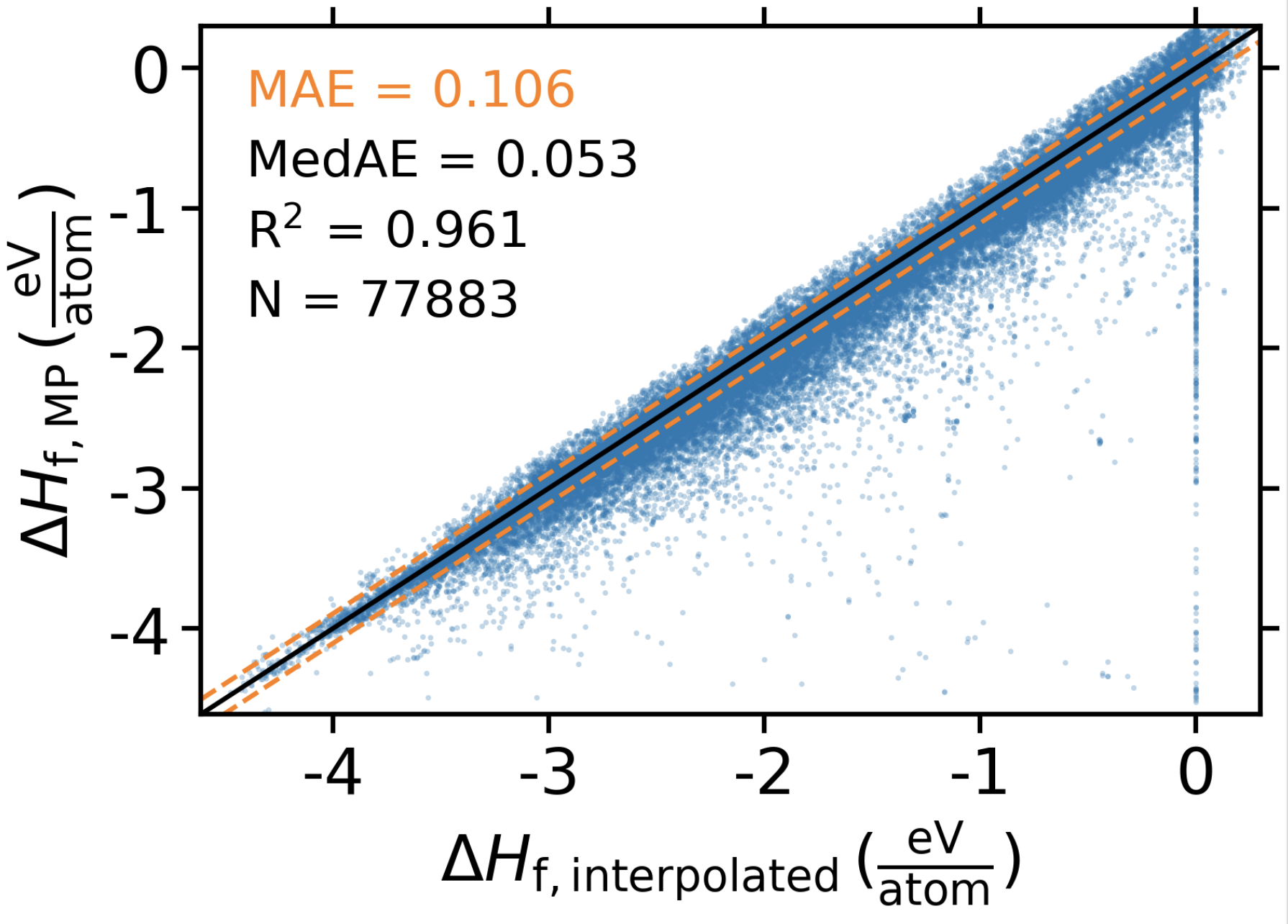
Leave-one-out validation of interpolation formation energies at \(0 K (\Delta H_f)\). MAE = mean absolute error (eV/atom). MedAE = median absolute error (eV/atom). N = number of materials evaluated.
Corrections to enthalpy values
Note that DFT systematically wrongly predicts the energies of certain ions. There is a correction method developed by pymatgen to correct this error, see pymatgen Compatibility. This method only applies to energies computed using PBE functionals.
In addition to the DFT corrections, we also fitted additional corrections for \(CO3^{2-}\) anions, which is \(-1.2485 ev/CO3\) in the current version. The details of this fitting could be find in the Jupyter notebook FixCO3.ipynb.
Finite-temperature Gibbs energy of formation interpolation
Once the zero-temperature formation enthalpy is calculated, we can approximate the finite-temperature thermodynamics, especially Gibbs energy of formation, using the methods developed in [ChrisNCOMM2018]. \(\Delta G_f(T)\) is calculated as:
\(\Delta G_f(T) = \Delta H_f(298K) + G_{SISSO}^\delta (T) - \sum_{i=1}^N \alpha_i G_i(T)\)
\(G_{SISS}^\delta (T) = (-2.48 \times 10^{-4} \cdot \ln (V) - 8.94 \times 10^{-5} m\cdot V^{-1})\cdot T + 0.181 \cdot \ln(T) - 0.882\)
Note that in the above equations, we use \(\Delta H_f(0K)\) to approximate \(\Delta H_f(298K)\), meaning that we ignore the effects of temperature and entropy on stability. Also, note that \(V\) is the volume of the compound, \(m\) is the reduced mass.
This enables us to determine reaction thermodynamics at temperatures relevant to a given synthesis reaction.
- ChrisNPJCOMPMATS2020
Bartel, Christopher J., et al. “A critical examination of compound stability predictions from machine-learned formation energies.” npj Computational Materials 6.1 (2020): 1-11.
- ChrisNPJCOMPMATS2019
Bartel, Christopher J., et al. “The role of decomposition reactions in assessing first-principles predictions of solid stability.” npj Computational Materials 5.1 (2019): 1-9.
- ChrisNCOMM2018
Bartel, Christopher J., et al. “Physical descriptor for the Gibbs energy of inorganic crystalline solids and temperature-dependent materials chemistry.” Nature communications 9.1 (2018): 1-10.
- SunSCIADV2016
Sun, Wenhao, et al. “The thermodynamic scale of inorganic crystalline metastability.” Science advances 2.11 (2016): e1600225.